x <- 0:20
y <- dpois(x, 5)
par(mar=c(5,5,4,2), cex.axis=1., cex.lab=1.)
plot(x, y, type='h', lwd=2, xlab="", ylab="Probability")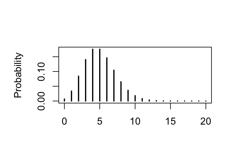
These are our object of study!
| Theoretical | Empirical | |
|---|---|---|
| e.g. Binomial, normal | \(\Longleftrightarrow\) | Observed data |
Statistical modeling considers how to bring these theoretical and the empirical pieces into correspondence.
Three ways to think about random variables:
Suppose we have a set of independent trials that each record a binary trial, where the probability of a positive outcome is \(p\).
We write these RVs as
\(X_1,\ldots, X_N \stackrel{i.i.d.}{\sim} \mathrm{Bernoulli}(p).\)
IDENTICAL: All trials are the same.
INDEPENDENT:
\(\mathbb{P}(X_i=k, X_j=r)=\mathbb{P}(X_i=k)\cdot \mathbb{P}(X_j=r)\)
Then:
\[ Y=\sum_{i=1}^N X_i \sim \mathrm{Binomial}(N,p). \]
Which also means:
\[ X\sim \mathrm{Binomial}(1,p)\equiv \mathrm{Bernoulli}(p). \]
One of our most common RVs is the binomial random variable:
\[ X\sim \mathrm{Binomial}(N,p) \Longleftrightarrow \mathbb{P}(X=k)=\binom{N}{k}\,p^k(1-p)^{N-k}. \]
As an abstract experiment: we can think of the binomial as \(N\) independent trials with binary (0/1) outcomes added together. Each trial has the same weight (\(p\)), the probability of a success.
Examples
Suppose \(X \sim \mathrm{Binomial}(N,p)\) and we observe that \(X=k\). A natural estimate for \(p\) is then
\[ \widehat{p}=\frac{k}{N}. \]
The probability mass function (pmf) gives the probability of a discrete random variable taking a value.
Binomial PMF:
\[ X\sim \mathrm{Poisson}(\lambda)\ \text{for}\ X=0,1,2,\ldots \Longleftrightarrow \mathbb{P}(X=k)=\frac{e^{-\lambda}\lambda^k}{k!}. \]
x <- 0:20
y <- dpois(x, 5)
par(mar=c(5,5,4,2), cex.axis=1., cex.lab=1.)
plot(x, y, type='h', lwd=2, xlab="", ylab="Probability")
Poisson random variables have a remarkable and statistically important property:
They can be added and they are still Poisson!
In math: If \(X\) and \(Y\) are independent and
\[ X \sim \mathrm{Poisson}(\mu) \quad\text{and}\quad Y \sim \mathrm{Poisson}(\lambda), \]
then
\[ X + Y \sim \mathrm{Poisson}(\mu + \lambda). \]
Continuous random variables take continuous values. Consequently, the concept of probabilistic mass no longer works and we need to consider probability density. It’ll be easiest to see this in context, so let’s consider a specific example — the exponential random variable.
Exponential random variable
\[ X \sim \mathrm{Exponential}(\lambda) \Longleftrightarrow f_X(x) = \lambda e^{-\lambda x} \quad\text{for}\quad x \ge 0. \]
Notice that we write \(f_X(x) = \lambda e^{-\lambda x}\): this is the probability density function. This does not give the probability of an exponential RV for each \(x\); it gives the density of the random variable.
\[ \mathbb{P}(a \le X \le b) = \int_a^b f_X(x)\,dx. \]
So the probability of observing a value between \(5\) and \(10\) is
\[ \mathbb{P}(5 \le X \le 10) = \int_{5}^{10} \lambda e^{-\lambda x}\,dx. \]
One of the most common and important random variables is the normal random variable:
\[ X \sim \mathrm{Normal}(\mu,\sigma) \Longleftrightarrow f_X(x) = \frac{1}{\sqrt{2\pi}\sigma}\exp\!\left(-\frac{(x-\mu)^2}{2\sigma^2}\right), \quad x \in \mathbb{R}. \]
\[ X \sim \mathrm{Binomial}(N,p) \]
dbinom(k, N, p): computes \(\mathbb{P}(X=k)\)pbinom(k, N, p): computes \(\mathbb{P}(X \le k)\)rbinom(M, N, p): generates \(M\) random draws from \(\mathrm{Binomial}(N,p)\)qbinom(alpha, N, p): finds \(k\) so that \(\mathbb{P}(X \le k) = \alpha\)